One of my other interests besides cyber security is data science, specifically machine learning. Having went through the Stanford University machine learning course by Dr Andrew Ng, I felt that it has provided me with the technical knowledge to go further and look at how machine learning is applied in the real world.

To keep it simple for reader’s new to machine learning, I will use the most simple machine learning algorithm taught by Dr Andrew, univariate linear regression. Univariate linear regression is used to solve regression problems. For example, what is the housing price in accordance with the land size within the area. The input for this example will be land size and the output will be the housing price. When this model is trained finished, the user should be able to input a new land size that he/she is trying to sell and the model should provide a predicted price. 

To train a model, lots of data need to be used. What this algorithm does is that it will produce a linear relationship between two variables, for example, X and Y. How do we determine that this straight line is the “line of best fit”? We use a cost function, specifically a squared error function to determine the global minimum. If we only have a few data, using squared error function to manually calculate global minimum is possible. As the number of data increases, we will need to use an algorithm to get the global minimum. One such algorithms is gradient descent.

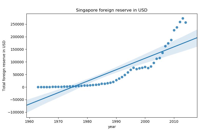
<Screenshot of the graph plotted using seaborn>

In this course, we used Octave to formulate the formula. Dr Ng himself mentioned that Octave is used for prototyping. I will use two methods to implement univariate linear regression. The first method is Python programming using Scikit-learn library. The second method is to use a free online tool called Microsoft Azure Machine Learning Studio. This tool does not require any programming to implement the machine learning model.

Before I start, let’s try to predict a value using real-world data. Singapore government has a website where they publish data (https://data.gov.sg/). One of the datasets is called Total Foreign Reserve in USD, with values ranging from 1963 to 2014. Because of the amount of data, I will use K-Fold cross validation. Head over to (Download CSV) to download the CSV file.

As a bonus, let’s try something interesting. Monetary Authority of Singapore website has published the official numbers from 2014 to 2018. (MAS Website). After we evaluate the model, we will use it to predict the values from 2015 to 2018 to see how much it varies.

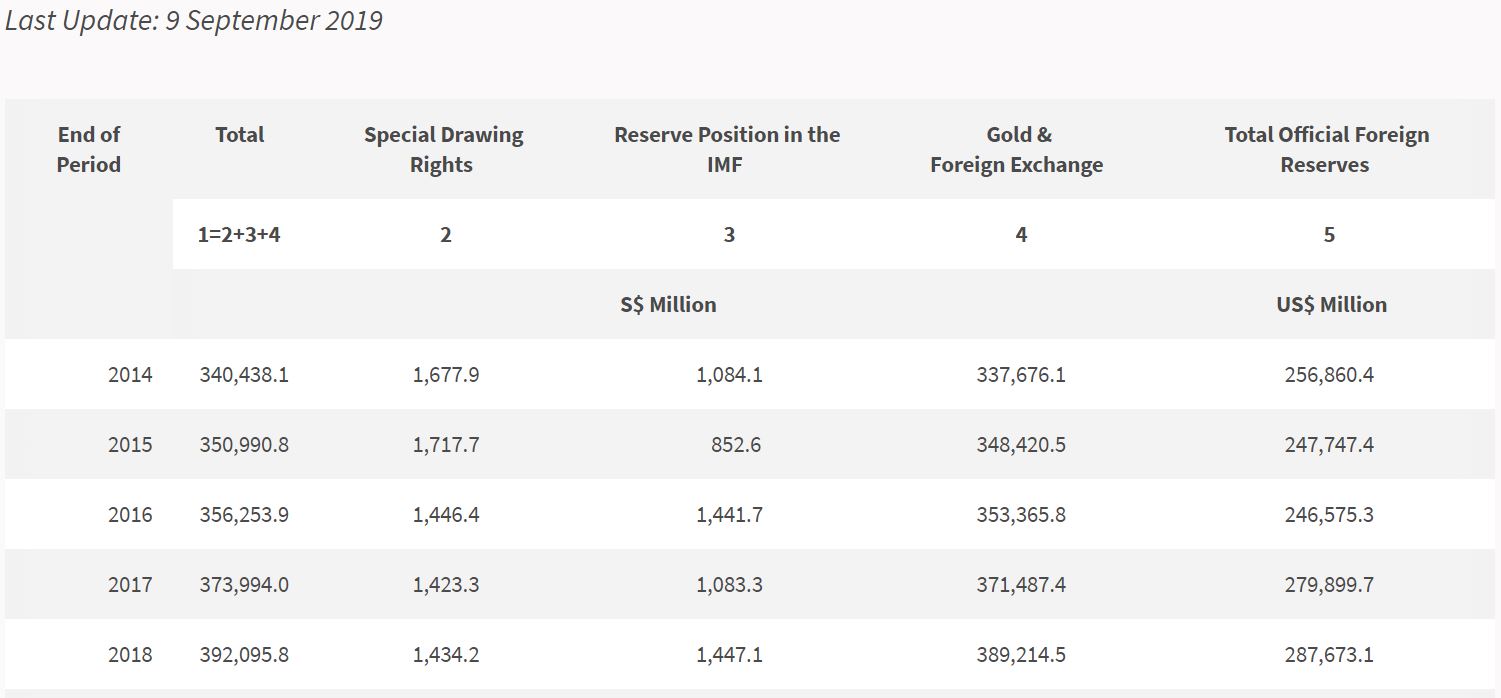
<Official Foreign Reserves. (n.d.). Retrieved October 1, 2019, from https://www.mas.gov.sg/statistics/reserve-statistics/official-foreign-reserves. Screenshot by author.>

Method One:

My preferred way to download Scikit-learn is to use Anaconda. Scikit-learn is an open source tool built on NumPy, SciPy and matplotlib. After installing Anaconda, install Scikit-learn using the CLI. The script for this project is available for download at Python Script.

Import the following libraries

import numpy 
import pandas
from sklearn.linear_model import LinearRegression
from sklearn.model_selection import KFold

This is the main portion of the script. First, we will read from the CSV file and create an empty array to store the score. Next, we will store the column values in X and y.

scores=[]
dataset = pandas.read_csv('total-foreign-reserves-annual.csv')

X = dataset['year'].values.reshape(-1,1)
y = dataset['total_foreign_reserve_usd'].values.reshape(-1,1)

Declare that linear regression is the learning algorithm. We will then set the KFold parameters. The first parameter is to split it into two groups, followed by shuffling the data randomly. At each iteration, the code will evaluate the score and store it inside the array. Finally, the code will display a mean R2 score of all the scores in the array.

clf = LinearRegression()
kf = KFold(n_splits=2, shuffle=True, random_state=40)
for train_index, test_index in kf.split(X):
    X_train, X_test = X[train_index], X[test_index]
    y_train, y_test = y[train_index], y[test_index]

    clf.fit(X_train, y_train)
    scores.append(clf.score(X_test, y_test))

print("The R2 Score for this model is: "+str(numpy.mean(scores)))

After running the code, we get an R2 Score of 0.75 (2 d.p). The higher the score for R2, the better it fits the data. There are no industry standards set for the required R2 scores. In fact, if an R2 score is too high, it could cause overfitting of data.

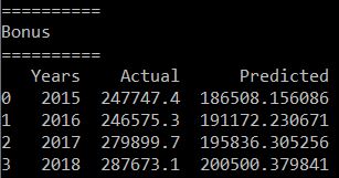
For this portion of the code is for the bonus. This is not a holdout cross validation but assuming that this model is created in 2014, how does the predicted values compared to the actual values.

# Bonus 
predict_years = numpy.array([[2015],[2016],[2017],[2018]], numpy.int32)
actual_years = numpy.array([[247747.4],[246575.3],[279899.7],[287673.1]], numpy.float_)

prediction = clf.predict(predict_years)

df = pandas.DataFrame({'Years': predict_years.flatten(),'Actual': actual_years.flatten(), 
	'Predicted': prediction.flatten()})
print(df)

The results of both the predicted and the actual ones are shown below. As you can see, the difference between the actual and predicted scores is getting greater and greater each year.

Method Two:

Head over to the URL https://studio.azureml.net/ This tool allows data of up to 10GB and comprises “drag and drop” components called items. This tool is powerful and simple to use. This is the closest experiment I can get to mirror the code above.
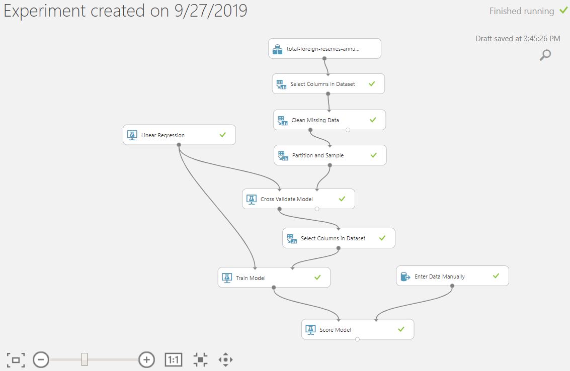
<Screenshot of my experiment on Azure Machine Learning Studio>

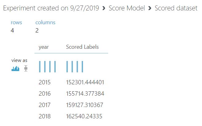
The result posted by Azure Machine Learning Studio differs from the ones posted by Scikit Learn. It is lower in comparison. <Screenshot of the results>

Conclusion:

The two methods used above are just a subset of the methods used in machine learning in the real world. Some other tools include Tensorflow, OpenML,Google Cloud AutoML, etc. Both tools are built for different audiences. As an introductory tool Azure Machine Learning Studio is an excellent tool to get into machine learning. In fact, I built my first model using this tool. Scikit Learn is quick as it runs locally on the computer and allows you to train model without an internet connection.

Now, let’s talk about the results. The limitations of univariate linear regression are evident here. By only taking the year into factor, we cannot create a model that can better predict the values. There are a lot of other machine learning algorithms we can try out there to find the one that best fits this data, but this is beyond this blog.

Credits:

[Contains information from Total Foreign Reserves accessed on 30/09/2019 from https://data.gov.sg/dataset/total-foreign-reserves which is made available under the terms of the Singapore Open Data Licence version 1.0 https://sg-mdh.mpa.gov.sg/content/singapore-open-data-licence-version-10]*